PyTree integrations

PyTrees are a powerful mechanism for working with nested data structures, while allowing algorithms like finite-differences, minimization, and integration routines to run on flattened 1D arrays of the the same data. To use PyTrees with vector objects, you need to install the optree package, and then register vector with PyTrees, for example:

import vector

pytree = vector.register_pytree()

state = {
    "position": vector.obj(x=1, y=2, z=3, t=0),
    "momentum": vector.obj(x=0, y=10, z=0, t=14),
}
flat_state, treedef = pytree.flatten(state)

flat_state is now a 1D array of length 8, and treedef contains the information needed to reconstruct the original structure:

print(flat_state)
print(treedef)

[0, 10, 0, 14, 1, 2, 3, 0]
PyTreeSpec({'momentum': CustomTreeNode(VectorObject4D[(<class 'vector.backends.object.VectorObject4D'>, <class 'vector.backends.object.AzimuthalObjectXY'>, <class 'vector.backends.object.LongitudinalObjectZ'>, <class 'vector.backends.object.TemporalObjectT'>)], [(*, *), (*,), (*,)]), 'position': CustomTreeNode(VectorObject4D[(<class 'vector.backends.object.VectorObject4D'>, <class 'vector.backends.object.AzimuthalObjectXY'>, <class 'vector.backends.object.LongitudinalObjectZ'>, <class 'vector.backends.object.TemporalObjectT'>)], [(*, *), (*,), (*,)])}, namespace='vector')

The original structure can be reconstructed with:

reconstructed_state = pytree.unflatten(treedef, flat_state)

Example: projectile motion with air resistance

In the following example, we use scipy.integrate.solve_ivp to solve the equations of motion for a projectile under the influence of gravity and air resistance.

To start, we wrap the solver, using PyTrees to flatten the state dictionary into a 1D array for the integrator, and then unflatten the result back into the original structure

from scipy.integrate import solve_ivp


def wrapped_solve(fun, t_span, y0, t_eval):
    flat_y0, treedef = pytree.flatten(y0)

    def flat_fun(t, flat_y):
        state = pytree.unflatten(treedef, flat_y)
        dstate_dt = fun(t, state)
        flat_dstate_dt, _ = pytree.flatten(dstate_dt)
        return flat_dstate_dt

    flat_solution = solve_ivp(
        fun=flat_fun,
        t_span=t_span,
        y0=flat_y0,
        t_eval=t_eval,
    )
    return pytree.unflatten(treedef, flat_solution.y)

Now, we set up the physical constants and initial conditions for the projectile motion problem, using the hepunits library to help us consistently track units throughout the calculation.

import numpy as np
import hepunits as u

gravitational_acceleration = vector.obj(x=0.0, y=-9.81) * (u.m / u.s**2)
air_density = 1.25 * u.kg / u.meter3
drag_coefficient = 0.47  # for a sphere
object_radius = 10 * u.cm
object_area = np.pi * object_radius**2
object_mass = 1.0 * u.kg

initial_position = vector.obj(
    x=0 * u.m,
    y=0 * u.m,
)
initial_momentum = (
    vector.obj(
        x=1 * u.m / u.s,
        y=20 * u.m / u.s,
    )
    * object_mass
)

The force function computes the total force on the object, including both gravity and air resistance. The tangent function then uses this to compute the time derivatives of position and momentum.

def force(position: vector.Vector2D, momentum: vector.Vector2D):
    gravitational_force = object_mass * gravitational_acceleration
    speed = momentum.rho / object_mass
    drag_magnitude = 0.5 * air_density * speed**2 * drag_coefficient * object_area
    drag_force = -drag_magnitude * momentum.unit()
    return gravitational_force + drag_force


def tangent(t: float, state):
    position, momentum = state
    dposition_dt = momentum / object_mass
    dmomentum_dt = force(position, momentum)
    return (dposition_dt, dmomentum_dt)

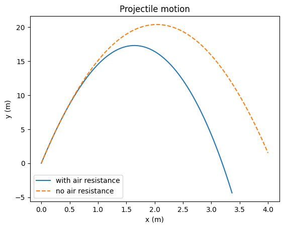
Finally, we solve the equations of motion using our wrapped solve_ivp, and plot the resulting trajectory alongside an analytic solution for projectile motion without air resistance.

time = np.linspace(0, 4, 100) * u.s

position, momentum = wrapped_solve(
    fun=tangent,
    t_span=(time[0], time[-1]),
    y0=(initial_position, initial_momentum),
    t_eval=time,
)

import matplotlib.pyplot as plt

fig, ax = plt.subplots()
ax.plot(position.x / u.m, position.y / u.m, label="with air resistance")

position_no_drag = (
    initial_momentum / object_mass * time + 0.5 * gravitational_acceleration * time**2
)

ax.plot(
    position_no_drag.x / u.m,
    position_no_drag.y / u.m,
    ls="--",
    label="no air resistance",
)

ax.set_xlabel("x (m)")
ax.set_ylabel("y (m)")
ax.set_title("Projectile motion")
ax.legend()

<matplotlib.legend.Legend at 0x120355fd0>